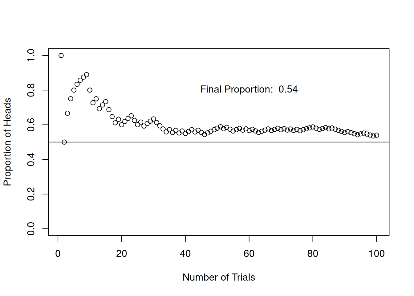
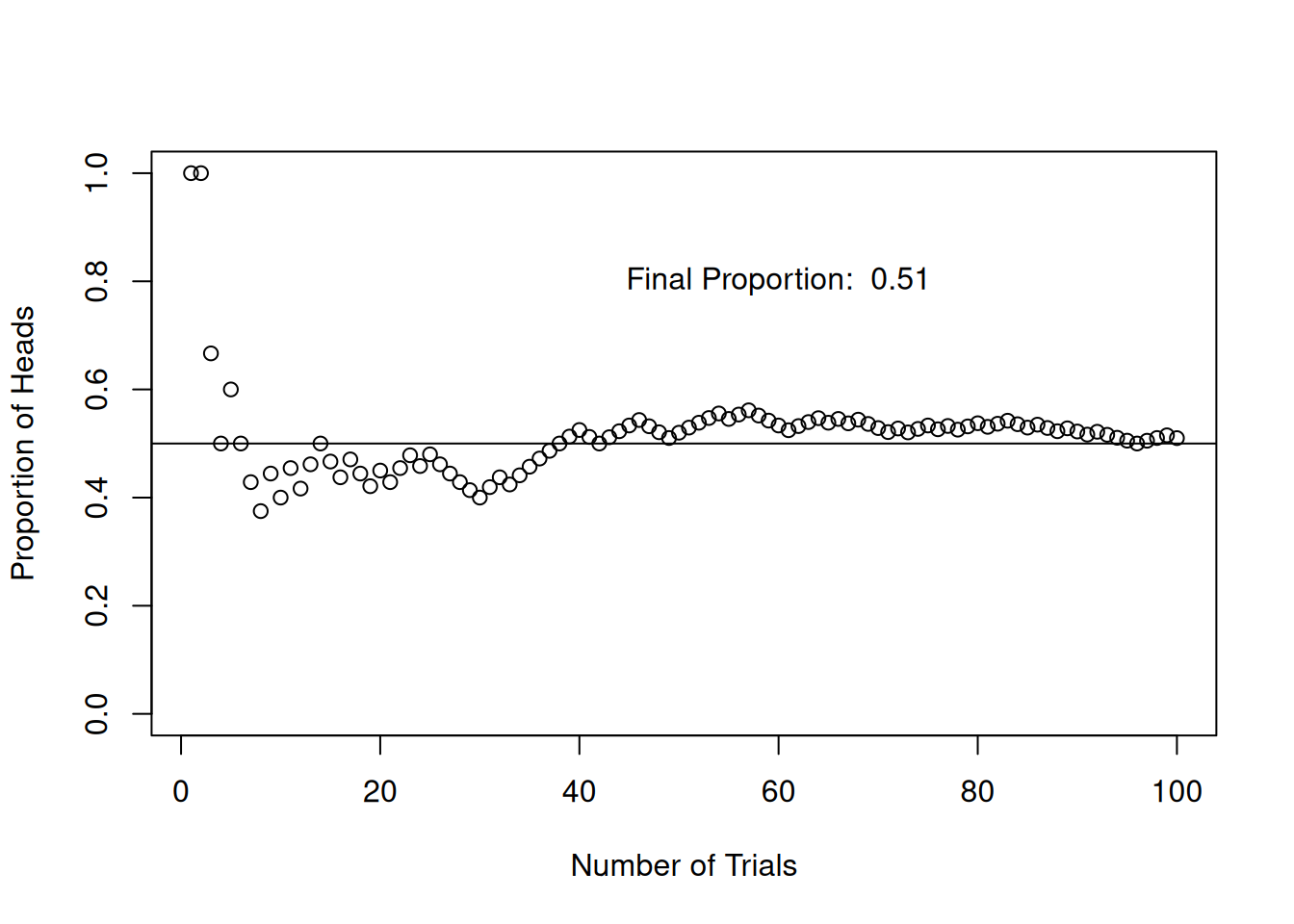
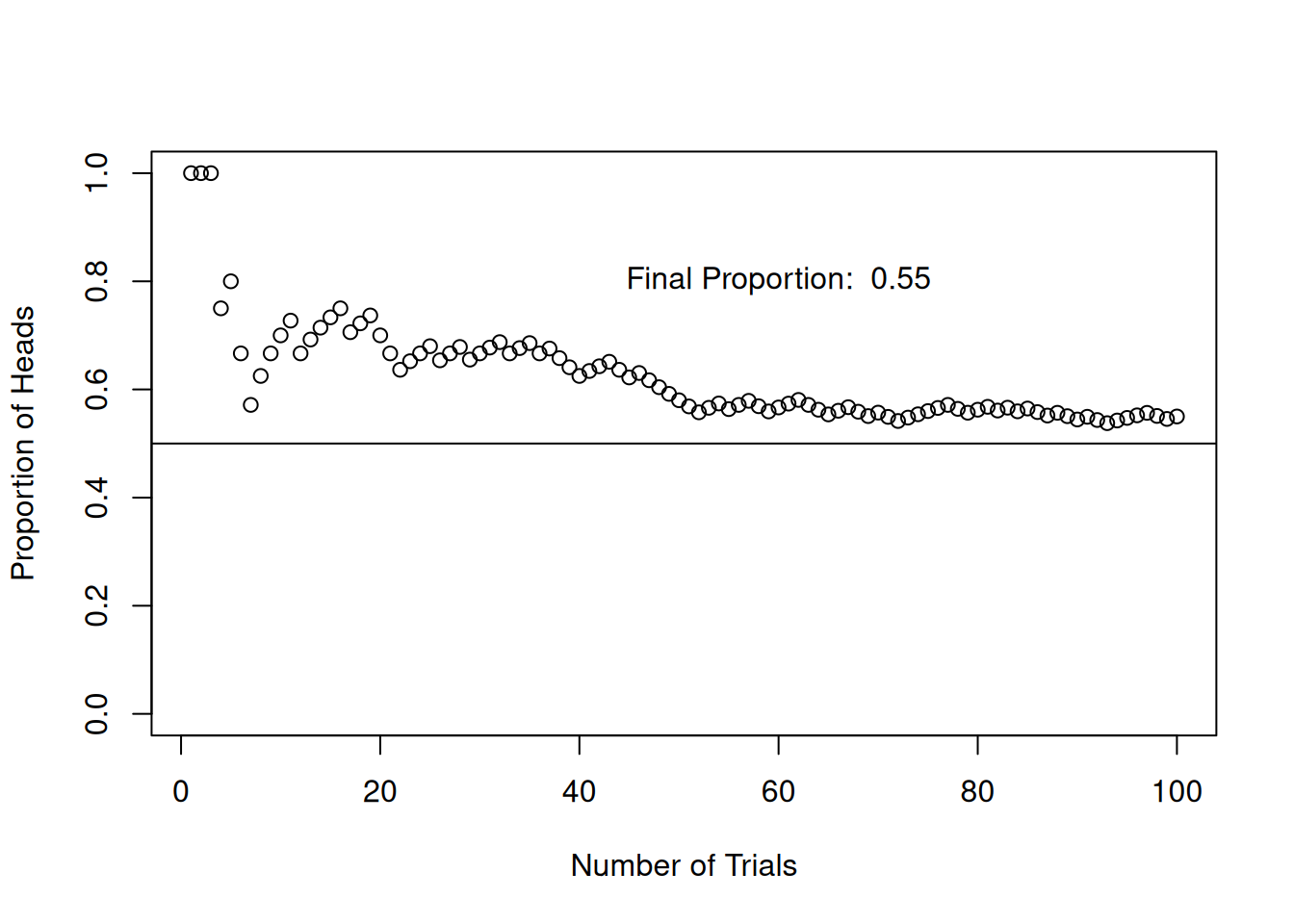
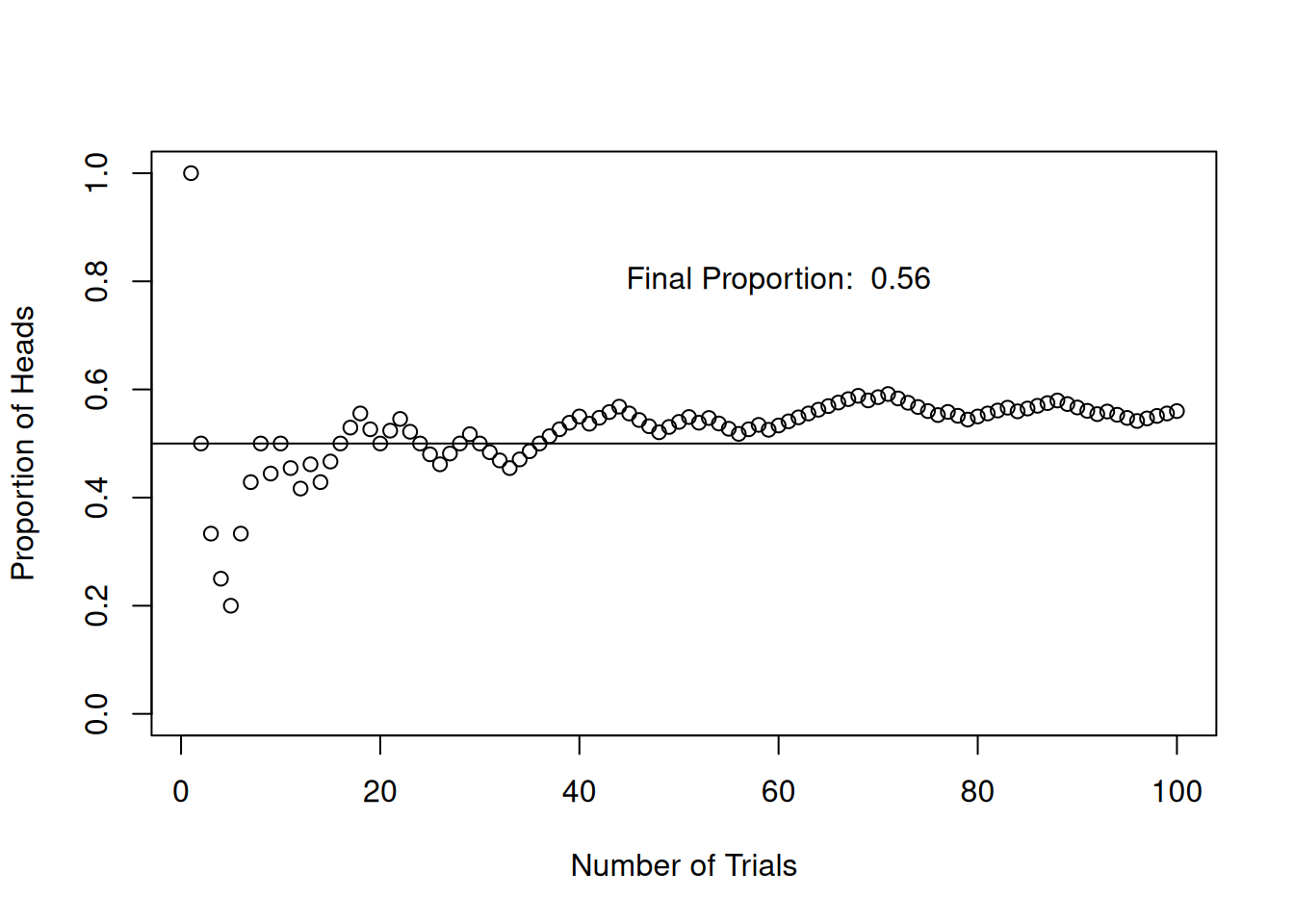
Flipping a coin is a probability experiment with two possible outcomes: heads(1), tails(0). Which outcome will occur when flipping the coin once cannot be predicted. The simulation is supposed to show what would happen if the experiment is repeated a lot of times.
Here we run the experiment in sets with 100 and 1000 repetitions (=trials). Each set will be repeated 4 times. The proportion of heads within the given number of trials will be determined after each trial. The results for the different sets will be plotted beside each other.
The Main Experiment
# run a loop 4 times to simulate the experiment with 100 trials 4 times for (v in1:4){# run the experiment 100 times (= 100 flips) and record the results (success = 1, failure = 0)# We can choose if success represent tails or heads. Here, for the rest of the process# we consider success to represent tails. records <-rbinom(100,1,0.5)# determine the cumulative number of heads after each flip cummulativeRecords <-cumsum(records)# determine the proportion of heads after each flip cummulativeProportion <- cummulativeRecords/c(1:length(records))# plot the proportion of heads against the number of trials plot(c(1:length(records)), cummulativeProportion, xlab="Number of Trials", ylab="Proportion of Heads", ylim=c(0,1))# add a line that represents the eassumed probability (= proportion) of heads # to show up after a lot of flipsabline(0.5, 0)# add some text, that displays the final proportion t <-paste("Final Proportion: ", cummulativeProportion[length(cummulativeProportion)])text(60, 0.8, t)}
Source Code
---title: "Flip a coin"description: "A simulation of the 'Flip a coin' experiment"date: "20240301"---## IntroductionFlipping a coin is a probability experiment with two possible outcomes: heads(1), tails(0). Which outcome will occur when flipping the coin once cannot be predicted. The simulation is supposed to show what would happen if the experiment is repeated a lot of times. Here we run the experiment in sets with 100 and 1000 repetitions (=trials). Each set will be repeated 4 times. The proportion of heads within the given number of trials will be determined after each trial. The results for the different sets will be plotted beside each other. ## The Main Experiment```{r}# run a loop 4 times to simulate the experiment with 100 trials 4 times for (v in1:4){# run the experiment 100 times (= 100 flips) and record the results (success = 1, failure = 0)# We can choose if success represent tails or heads. Here, for the rest of the process# we consider success to represent tails. records <-rbinom(100,1,0.5)# determine the cumulative number of heads after each flip cummulativeRecords <-cumsum(records)# determine the proportion of heads after each flip cummulativeProportion <- cummulativeRecords/c(1:length(records))# plot the proportion of heads against the number of trials plot(c(1:length(records)), cummulativeProportion, xlab="Number of Trials", ylab="Proportion of Heads", ylim=c(0,1))# add a line that represents the eassumed probability (= proportion) of heads # to show up after a lot of flipsabline(0.5, 0)# add some text, that displays the final proportion t <-paste("Final Proportion: ", cummulativeProportion[length(cummulativeProportion)])text(60, 0.8, t)}```