# (install &) load packages
pacman::p_load(
  broom,
  conflicted,
  modelbased,
  tidyverse)

# handle function conflicts
conflicts_prefer(dplyr::filter)
conflicts_prefer(dplyr::select)

# load data and change variable into the correct data type
path <- "https://raw.githubusercontent.com/SchmidtPaul/dsfair_quarto/master/data/Mead1993.csv"
dat <- read_csv(path) %>%
mutate(variety = as.factor(variety))One Way CRD Analysis
this is a reading note of this tutorial.
Load Data & Packages
Inspect the data
dat %>%
  group_by(variety) %>%
  dlookr::describe(yield) %>%
  select(2:sd, p00, p100) %>%
  arrange(desc(mean))
Registered S3 methods overwritten by 'dlookr':
method from
plot.transform scales
print.transform scales# A tibble: 4 × 7
variety n na mean sd p00 p100
<fct> <int> <int> <dbl> <dbl> <dbl> <dbl>
1 v2 6 0 37.4 3.95 32.0 43.3
2 v4 6 0 29.9 2.23 27.6 33.2
3 v1 6 0 20.5 4.69 15.9 26.4
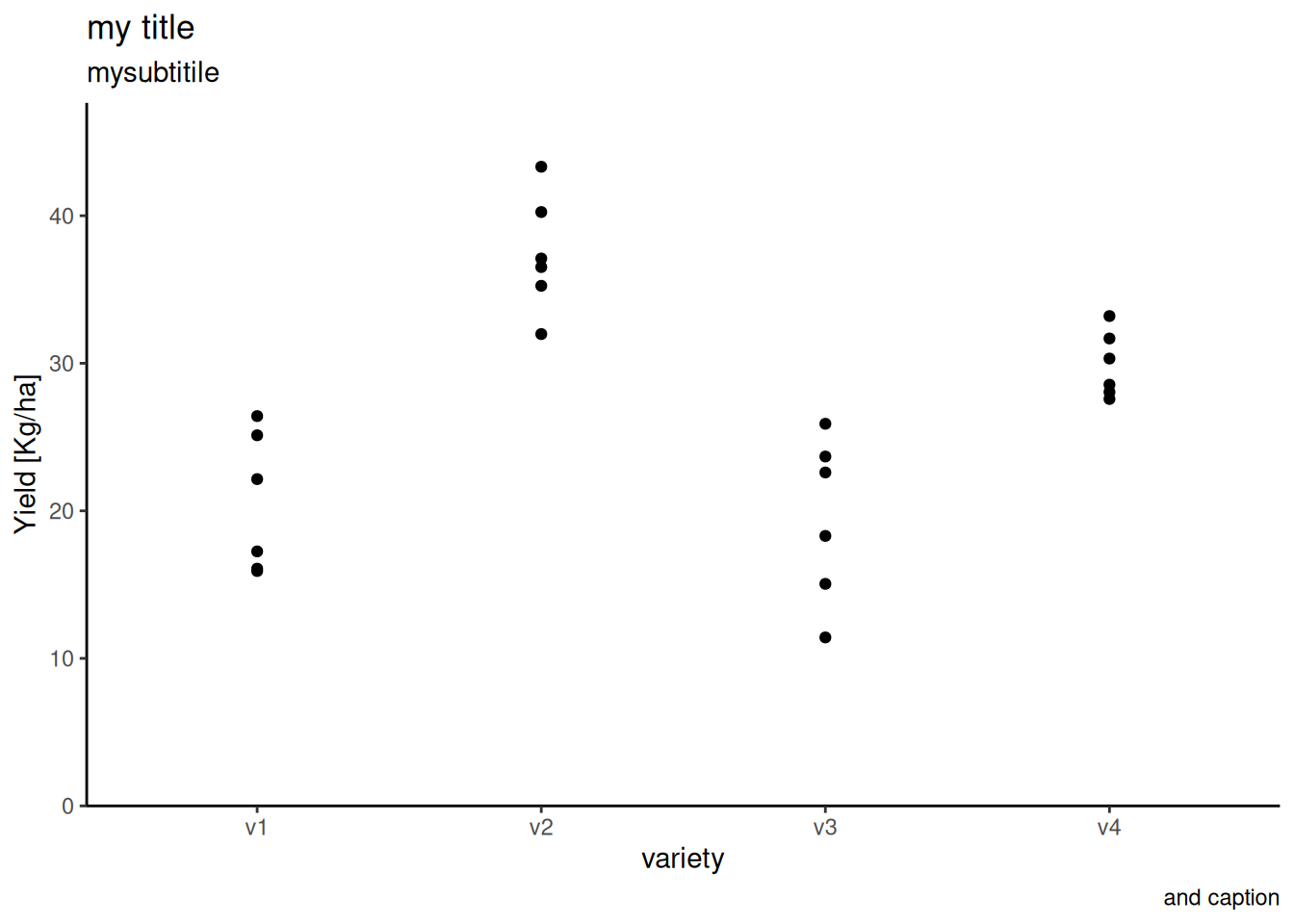
4 v3 6 0 19.5 5.56 11.4 25.9In the data, only “yield” is true numerial. “variety” is a factor and has 4 levels.
Below is the plot of the data.
ggplot(data = dat) +
  aes(y = yield, x = variety) +
  geom_point() +
  # ggtitle("Hello Test") +  # this a short cut function
  labs(
    title = "my title",
    subtitle = "mysubtitile",
    caption = "and caption"
  ) +
  # theme(
  #   axis.line.x = element_line(color = "green", linetype = "dotted")
  # )
  theme_classic() +
  scale_y_continuous(
    name = "Yield [Kg/ha]",
    limits = c(0, NA), # y-axis starts at 0 and ends at ggplot-default, i.e. the highest point.

    # fixed value is possible
    # expand = c(0, 0),

    expand = expansion(mult = c(0, 0.1)), # but defined dynamically is better
  )
Modelling
mod <- lm(yield ~ variety, data = dat)
mod
Call:
lm(formula = yield ~ variety, data = dat)

Coefficients:
(Intercept)    varietyv2    varietyv3    varietyv4
    20.4900      16.9133      -0.9983       9.4067
Since “variety” is a factor, instead of one single slope, we’ve got one estimate for the effect brought by each level. Here’s the interpretation of the coefficient of our lm model:
- Intercept – the baseline, which shows the yield of planting solely melon of variety 1 is \(20.49\) kg/ha.
- The rest of the value – the individual deviation for each further variety
A summary of prediction based on the model:
- pred of var 1: \(20.49 + 0 = 20.49\) kg/ha
- pred of var 2: \(20.49 + 16.9133 = 37.40\) kg/ha
- pred of var 3: \(20.49 - 0.9983 = 19.49\) kg/ha
- pred of var 4: \(20.49 + 9.4067 = 29.89\) kg/ha
AVOVA (F-test)
Null hypothesis H_0: no matter if var 1, var 2, var 3 or var 4 is chosen, the yield stays the same. Alternative hypothesis H_A: at least one of them makes difference.
anova(mod)Analysis of Variance Table
Response: yield
Df Sum Sq Mean Sq F value Pr(>F)
variety 3 1291.48 430.49 23.418 9.439e-07 ***
Residuals 20 367.65 18.38
---
Signif. codes: 0 '***' 0.001 '**' 0.01 '*' 0.05 '.' 0.1 ' ' 1Since \(p < 0.001\), we believe it’s extreme unlikely to find a sample that support the null hypothesis. Thus we believe in with the alternative hypothesis instead, i.e. our lm model has statistic significance.